gamson <- read_rds("data/gamson.rds")

ggplot(gamson, aes(x = seat_share, y = portfolio_share)) +
  geom_point() +
  geom_smooth()
To fit a regression model in R, we can use the following approach:
lm() to fit the model.coef(), arm::display(), modelsummary::modelsummary, or summary() to quickly inspect the slope and intercept.geom_smooth()In the context of ggplot, we can show the fitted line with geom_smooth().
gamson <- read_rds("data/gamson.rds")
ggplot(gamson, aes(x = seat_share, y = portfolio_share)) +
geom_point() +
geom_smooth()
By default, geom_smooth() does two things we don’t want:
method = "lm" to geom_smooth().se = FALSE to geom_smooth().ggplot(gamson, aes(x = seat_share, y = portfolio_share)) +
geom_point() +
geom_smooth(method = "lm", se = FALSE)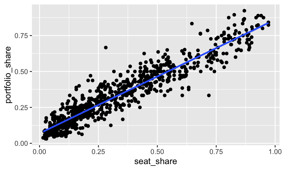
In the case of Gamson’s law, the line \(y = x\) is theoretically relevant. It’s not the regression line, it’s the line that indicates a perfectly proportional portfolio distribution. To include it, we can use geom_abline().
ggplot(gamson, aes(x = seat_share, y = portfolio_share)) +
  geom_point() +
geom_smooth(method = "lm", se = FALSE) +
geom_abline(intercept = 0, slope = 1, color = "red")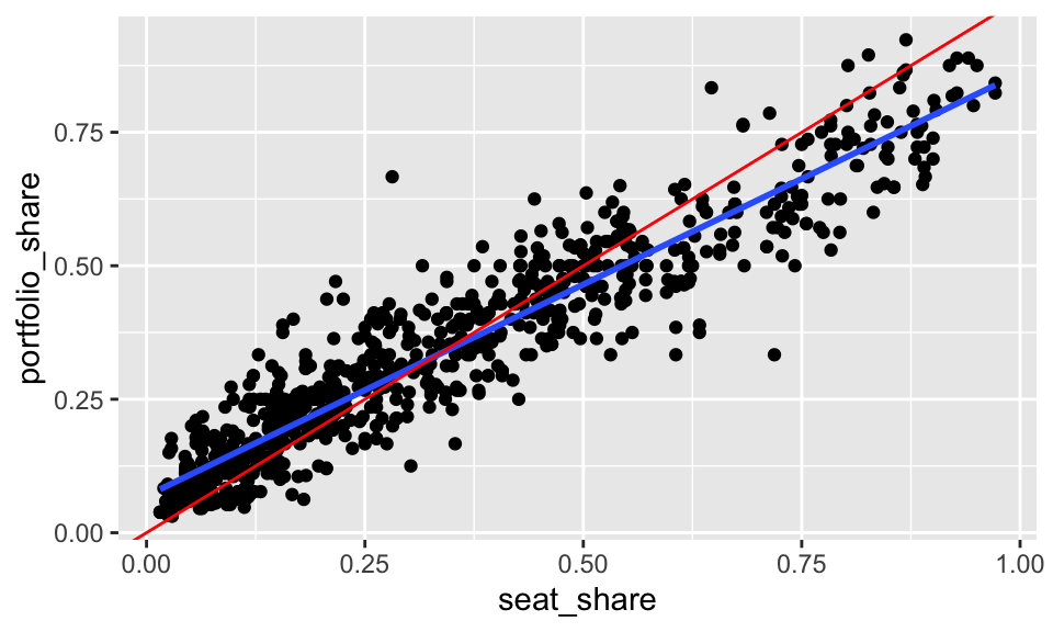
lm()The lm() function takes two key arguments.
~. You put the name of the outcome variable \(y\) on the LHS and the name of the explanatory variable \(x\) on the RHS. (We haven’t seen this yet, but it’s common to have multiple variables on the RHS like y ~ x1 + x2 + x3.)fit <- lm(portfolio_share ~ seat_share, data = gamson)We have several ways to look at the fit. Experiment with coef(), arm::display(), modelsummary::modelsummary(), and summary() to see the differences. For now, we only understand the slope and intercept, so coef() works perfectly.
coef(fit)(Intercept) seat_share
0.06913558 0.79158398 The coef() function outputs a numeric vector with named entries. The intercept is named (Intercept) and the slope is named after its associated variable.
Experiment with the others!
# a bit more detail
arm::display(fit)

# a lot more detail
summary(fit)

# exports to a lot of different formats, see help file
modelsummary::modelsummary(fit)Exercise 1
anscmobe dataset into R. Download from here if needed. Use glimpse(anscombe) to get a quick look at the data. Realize that this one data frame actually contains four different datasets stacked on top of each other and numbered I, II, III, and IV.filter() the dataset before supplying the data to lm() or use can supply the subset argument to lm(). In this case, just supplying subset = dataset == "I", for example, is probably easiest. Fit the regression to all four datasets and put the intercept, slope, RMS of the residuals, and number of observations for each regression in a little table. Interpret the results.Exercise 2
Use regression to test Clark and Golder’s (2006) theory using the parties dataset we’ve seen before (from here). First, create scatterplots between ENEG and ENEP faceted by the electoral system with with the least-squares fit included in each. Then fit three separate regression models. Fit the model \(\text{ENEP}_i = \alpha + \beta \text{ENEG}_i + r_i\) for SMD systems, small-magnitude PR systems, and large-magnitude PR systems. Include the intercept, slope, and RMS of the residuals from each fit in a little table. Explain the results. Explain any inadequacies of the regression model (from the scatterplots).
Exercise 3
Get the economic-models.csv dataset here. You can find all the details here.
Use tables and figures wisely to answer the questions above.