# a collection of numbers (that we'll sample from below)
collection <- c(-2, -1, 0, 1, 2)

# take one sample from the collection
sample(collection, size = 1)
[1] -1In the previous chapter, we showed that the difference-in-means estimator \(\widehat{\text{ATE}} = \overline{Y}^{\text{obs}}_{t} - \overline{Y}^{\text{obs}}_{c}\) is an unbiased estimator of the average treatment effect. Unbiasedness tells us that our estimator gets it right on average in the long-run.1
1 Remember that “long run” means that we are repeatedly re-randomizing many, many times. Each randomization gives us a different collection of observed outcomes (i.e., one per respondent).
But unbiasedness is only part of the story. An estimator can be unbiased yet still produce estimates that are far from the true value in any given experiment. What we need to understand is how much our estimate varies from one randomization to another. We want our procedure to produce an estimate that is right on average AND usually close to the ATE. The variance of the estimator tells us how close the estimate falls to the ATE in the long run.
In this chapter, we state the variance formula for \(\widehat{\text{ATE}}\) under completely randomized experiments and explain what it means. The proof, which involves very tedious algebra (but only tedious algebra), appears in Appendix A.
Understanding this variance formula will help us understand the noisiness of our estimates and think carefully about how to design experiments.
The variance operator \(\text{Var}[\cdot]\) is a way of measuring “how spread out” a random variable is around its average value. The variance of a random variable measures its typical squared distance from the mean.
Rule: Variance is defined as the expected squared deviation from the mean.
If \(X\) is random, then
\[ \text{Var}(X) = E\left[(X - E[X])^2\right]. \]
Notice the logic. We’re just computing the long-run average of \((X - E[X])^2\), which is the squared difference between \(X\) and its own long-run average.
It also turns out that
\[ \text{Var}(X) = E\left[X^2 \right] - \left(E[X]\right)^2, \]
which can be a little easier to work with, but is somewhat harder to conceptualize.
A simulation helps illustrate. Suppose we sample once from the collection -2, -1, 0, 1, 2. This single sample is random—it might be -2, -1, 0, 1, or 2 with equal probability.
# a collection of numbers (that we'll sample from below)
collection <- c(-2, -1, 0, 1, 2)
# take one sample from the collection
sample(collection, size = 1)[1] -1What’s the variance of this sample?
We can take 100,000 samples x from this collection and compute mean((x - mean(x))^2). In this case, 100,000 is long enough approximate the “long run.”
# take and store many (approximating long-run) samples from the collection (with replacement)
x <- sample(collection, size = 100000, replace = TRUE)

# compute variance in several steps
avg <- mean(x)
sq_dev <- (x - avg)^2
mean(sq_dev)  # avg squared deviation
[1] 2.00787# compute in one step
mean((x - mean(x))^2)[1] 2.00787We don’t need a computer to approximate the variance; we can use our knowledge of expected values to find it exactly. We can compute it most easily using the definition \(\text{Var}(X) = E\left[X^2 \right] - \left(E[X]\right)^2\) mentioned in the aside above.
Let \(X\) be a random variable that takes values in \(\{-2,-1,0,1,2\}\) with equal probability \(1/5\). This is what the code is doing when it samples x.
We need to compute both \(E\left[X^2 \right]\) and \(\left(E[X]\right)^2\). Let’s start with the second, because it’s easier.
First compute \(E[X]\). This is easy.
\[ E[X] = \frac{1}{5}(-2 - 1 + 0 + 1 + 2) = 0. \]
Since \(E[X] = 0\), \(E[X]^2 = 0\) and the second term on the right-hand side drops out.
Next, compute \(E\left[X^2 \right]\).
\[ E[X^2] = \frac{1}{5}\left( (-2)^2 + (-1)^2 + 0^2 + 1^2 + 2^2 \right) = \frac{10}{5} = 2. \]
Therefore, \[ \text{Var}(X) = E\left[X^2 \right] - \left(E[X]\right)^2 = 2 - 0 = 2. \]
Now that we understand how variance measures the spread of a random variable, we can state the variance of our estimator \(\widehat{\text{ATE}}\). Remember, because we are choosing to randomly assign participants to treatment and control, our procedure produces a random estimate.
Under completely randomized assignment, the variance of \(\widehat{\text{ATE}}\) is
\[ \text{Var}_D \left(\widehat{\text{ATE}}\right) = \frac{S_t^2}{N_t} + \frac{S_c^2}{N_c} - \frac{S_{tc}^2}{N}, \]
where \(S_t^2\) is defined as
\[ S_t^2 = \frac{1}{N - 1} \sum_{i=1}^{N} (Y_i(1) - \overline{Y}(1))^2 \quad \text{and}, \]
\(S_c^2\) is defined as
\[ S_c^2 = \frac{1}{N - 1} \sum_{i=1}^{N} (Y_i(0) - \overline{Y}(0))^2, \]
and \(S_{tc}^2\) is defined as
\[ S_{tc}^2 = \frac{1}{N - 1} \sum_{i=1}^{N} \left(\tau_i - \text{ATE}\right)^2. \]
Somewhat (or perhaps very) confusingly, \(S_t^2\), \(S_c^2\), and \(S_{tc}^2\) are also called “variance.” We use the variance \(\text{Var}(X) = E\left[(X - E[X])^2\right]\) to describe the spread of random numbers (like noisy estimates) and the variances \(S_t^2\), \(S_c^2\), and \(S_{tc}^2\) to describe the spread of a fixed collection of numbers (like potential outcomes under treatment). Statisticians sometimes call the latter finite population variances to distinguish them.
You may notice that \(S_t^2\), \(S_c^2\), and \(S_{tc}^2\) are defined with \(1/(N-1)\) in the denominator rather than \(1/N\). This follows the convention used by Cochran (1977) and later adopted by Imbens and Rubin (2015).
This choice differs from the arguably more “elementary” variance
\[ V_N = \frac{1}{N} \sum_{i=1}^N (x_i - \bar{x})^2, \]
which is often introduced in introductory texts and interpretable as the average squared deviation from the mean.
The \(1/(N-1)\) convention has a key advantage: it aligns the definition of the population variance with the sample variance estimator, so that sample variances are unbiased estimators of population variances. This simplifies the algebra of variance estimation in randomized experiments. While readers accustomed to the \(1/N\) normalization may find this convention unfamiliar, for design-based inference—where randomness arises from treatment assignment—the \(1/(N-1)\) normalization offers conceptual and algebraic advantages.
Let’s unpack this formula.
Before interpreting the formula, let’s understand what each quantity measures. \(S_t^2\) measures how spread out the potential outcomes under treatment are across individuals. \(S_c^2\) measures the same for control. And \(S_{tc}^2\) measures how spread out the individual treatment effects are—that is, how much the treatment effect varies from person to person.
The variance formula has three terms.
Term 1: \(\frac{S_t^2}{N_t}\) This is the variance of the treatment group mean. If potential outcomes under treatment vary a lot across individuals (large \(S_t^2\)), our estimate of the treatment group mean will be more variable. Dividing by \(N_t\) reflects that larger treatment groups give us more precise estimates.
Term 2: \(\frac{S_c^2}{N_c}\) Similarly, this is the variance of the control group mean. More variability in control potential outcomes or fewer control individuals increases variance.
Term 3: \(-\frac{S_{tc}^2}{N}\) This is the interesting (and difficult) term. Importantly, it shrinks the variance. The quantity \(S_{tc}^2\) measures how variable the individual treatment effects are. If everyone has the same treatment effect (constant effects), then \(S_{tc}^2 = 0\) and this term disappears.
When treatment effects are constant (every individual experiences the same effect \(\tau\)), we have \(\tau_i = \tau\) for all \(i\). In this case, something remarkable happens: \(S_{tc}^2 = 0\). In this case, the variance simplifies to
\[ \text{Var}_D \left(\widehat{\text{ATE}}\right) = \frac{S_t^2}{N_t} + \frac{S_c^2}{N_c}. \]
Moreover, when effects are constant, \(S_t^2 = S_c^2 = S^2\) (the variance of potential outcomes is the same under treatment and control), so
\[ \text{Var}_D \left(\widehat{\text{ATE}}\right) = S^2 \left(\frac{1}{N_t} + \frac{1}{N_c}\right). \]
This is the familiar variance formula you might have seen in an introductory statistics course for the difference of two means.
The algebraic proof of the variance formula is long, but the intuition of the result is straightforward.
The variance of \(\widehat{\text{ATE}}\) reflects how much our estimate would change if we repeated the same experiment many times.2
2 Remember all that changes across these many repetitions is who is assigned to treatment and control. Every randomization produces a slightly different treatment group and a slightly different control group, and therefore a slightly different estimate of the ATE.
There are two obvious reasons why \(\widehat{\text{ATE}}\) varies across repetitions.
Randomness in the treatment-group mean. Different randomizations place different individuals into the treatment group. Since individuals have different potential outcomes under treatment, the treatment-group mean \(\overline{Y}^{\text{obs}}_t\) will not be exactly the same every time. The amount it varies depends on the spread of the potential outcomes (\(S_t^2\)) and the number of individuals assigned to treatment (\(N_t\)). This produces the term \(\frac{S_t^2}{N_t}\).
Randomness in the control-group mean. The same logic applies to the control group. Different randomizations create different control groups, so the control-group mean also varies in the same way as the treatment group.
If these two sources of variation were unrelated, the variance of \(\widehat{\text{ATE}}\) would simply be the sum of these two terms. However, they are not unrelated. They are related in a subtle, interesting, and important way.
Each individual can be in only one group. If someone is assigned to treatment, they cannot be assigned to control. This creates a link between the two group means.
To understand why this matters, focus on an individual with an unusually large treatment effect. For this person, the difference between their treated outcome \(Y_i(1)\) and their control outcome \(Y_i(0)\) is especially large.3
3 To make this even more concrete, we might imagine this person’s potential outcomes are among the largest under treatment and among the smallest under control.
Now consider what happens when this individual is assigned to the treatment group. Their treated outcome \(Y_i(1)\) is relatively high, so their presence pushes the treatment-group mean upward.
But assigning them to treatment also means they are missing from the control group. Because their treatment effect is unusually large, their control outcome \(Y_i(0)\) is relatively low. Had they been assigned to control, their low outcome would have pulled the mean of the control-group downward. Since they are not in the control group, that downward pull doesn’t happen.
As a result, two things happen.
These effects partially cancel out when we take the difference between the treatment and control group.
This stabilizing effect comes specifically from individuals with unusually large (or unusually small) treatment effects. Individuals with “typical” treatment effects do not create this cancelling dynamic. The more treatment effects vary across people, the stronger this stabilizing effect becomes. That variation is exactly what \(S_{tc}^2\) measures.
This is why the variance formula includes the negative term \(-\frac{S_{tc}^2}{N}\).
And then, if treatment effects are constant, then no one has unusually large (or unusually small) treatment effect and the cancelling dynamic is absent.
Let’s verify the variance formula with a simulation. We’ll create a small population of 10 individuals with known potential outcomes, compute the theoretical variance using the formula, and then simulate 1,000 randomizations to see if the simulated variance matches.
First, we create potential outcomes for 10 individuals. We’ll use the same hypothetical data from the previous chapters.
# load packages
library(tidyverse)

# create potential outcomes for 10 individuals
po <- tibble(
  i = 1:10,
  Y0 = c(4, 6, 5, 3, 7, 5, 4, 6, 5, 4),  # potential outcome under control
  Y1 = c(7, 5, 5, 9, 10, 4, 8, 7, 3, 6)  # potential outcome under treatment
)

# compute individual treatment effects
po <- po |>
  mutate(tau = Y1 - Y0)

# view the data
po
# A tibble: 10 × 4
i Y0 Y1 tau
<int> <dbl> <dbl> <dbl>
1 1 4 7 3
2 2 6 5 -1
3 3 5 5 0
4 4 3 9 6
5 5 7 10 3
6 6 5 4 -1
7 7 4 8 4
8 8 6 7 1
9 9 5 3 -2
10 10 4 6 2Now we compute the quantities we need for the variance formula.
# sample size and group sizes
N <- 10
N_t <- 5
N_c <- 5

# compute means of potential outcomes
Y1_bar <- mean(po$Y1)
Y0_bar <- mean(po$Y0)

# compute the true ATE
ATE <- Y1_bar - Y0_bar
ATE
[1] 1.5Next, we compute \(S_t^2\), \(S_c^2\), and \(S_{tc}^2\).
# variance of Y(1)
S_t_sq <- var(po$Y1)
S_t_sq
[1] 4.933333# variance of Y(0)
S_c_sq <- var(po$Y0)
S_c_sq[1] 1.433333# variance of treatment effects
S_tc_sq <- var(po$tau)
S_tc_sq[1] 6.5Using the variance formula, we compute the theoretical variance of \(\widehat{\text{ATE}}\).
# theoretical variance using the formula
theoretical_var <- S_t_sq / N_t + S_c_sq / N_c - S_tc_sq / N
theoretical_var
[1] 0.6233333Now we simulate 1,000 randomizations and compute \(\widehat{\text{ATE}}\) for each one. We use a simple for-loop to make the logic clear.
# set seed for reproducibility
set.seed(1234)

# number of simulations
n_sims <- 1000

# create a vector to store the estimates
ate_estimates <- numeric(n_sims)

# run the simulation
for (sim in 1:n_sims) {

 # randomly assign 5 individuals to treatment
  treated <- sample(1:N, size = N_t, replace = FALSE)

  # compute observed outcomes
  Y_obs_t <- po$Y1[treated]       # treated individuals show Y(1)
  Y_obs_c <- po$Y0[-treated]      # control individuals show Y(0)

  # compute the estimate for this randomization
  ate_estimates[sim] <- mean(Y_obs_t) - mean(Y_obs_c)
}Finally, we compare the theoretical variance to the variance of our simulated estimates.
# simulated variance
simulated_var <- var(ate_estimates)

# compare the two
tibble(
  theoretical_variance = theoretical_var,
  simulated_variance = simulated_var,
)
# A tibble: 1 × 2
theoretical_variance simulated_variance
<dbl> <dbl>
1 0.623 0.552The simulated variance is very close to the theoretical variance. The small difference is due to simulation error. With more simulations, the two values would converge.
We can also visualize the distribution of estimates.
ggplot(tibble(ate = ate_estimates), aes(x = ate)) +
  geom_histogram(binwidth = 0.25, fill = "grey80") +
  geom_vline(xintercept = ATE) +
  theme_minimal()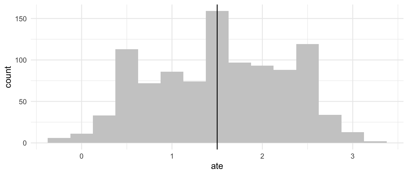
Unbiasedness means that the estimator is correct on average. If we could repeat the experiment many times with different randomizations, the average of all our estimates would equal the true ATE. But any single estimate might be far from the truth.
Low variance means that the estimates are tightly clustered around their average value. Different randomizations produce similar estimates.
Yes, an estimator can be unbiased but still give poor estimates in practice. Imagine an estimator that, across many randomizations, produces estimates of \(-100\) half the time and \(+102\) half the time (when the true ATE is 1). This estimator is unbiased (the average is 1), but any single estimate is wildly wrong.
In practice, we want both properties: an estimator that is unbiased and has low variance. The ideal estimator hits close to the target on average (unbiased) and doesn’t scatter too much around that average (low variance).
First term (\(S_t^2/N_t\)): This represents the uncertainty in estimating the average treatment group outcome. \(S_t^2\) measures how much the potential outcomes under treatment vary across individuals. When there’s more variation, the particular individuals who happen to land in the treatment group could have very different outcomes from another randomization. Dividing by \(N_t\) reflects that larger treatment groups give more stable estimates.
Second term (\(S_c^2/N_c\)): Similarly, this represents the uncertainty in estimating the average control group outcome. It depends on how variable the control potential outcomes are and how many individuals are in the control group.
Third term (\(-S_{tc}^2/N\)): This term reduces the variance, which seems surprising at first. Here \(S_{tc}^2\) is the variance of the individual-level treatment effects \(\tau_i = Y_i(1) - Y_i(0)\). It measures how much treatment effects vary across individuals. Formally,
\[ S_{tc}^2 = \frac{1}{N-1} \sum_{i=1}^{N} (\tau_i - \text{ATE})^2. \]
The third term captures the fact that treatment and control group assignments are not independent. They are negatively correlated. If one individual goes to treatment, another must go to control.
The negative sign arises because treatment and control assignments are linked. When a high-treatment-effect individual is assigned to treatment, they are necessarily missing from control. This creates a stabilizing dynamic: the treatment mean goes up (because they have high \(Y(1)\)), but so does the control mean (because their low \(Y(0)\) is absent). The difference between the means is more stable than either mean alone. This stabilizing effect is stronger when treatment effects are more heterogeneous (larger \(S_{tc}^2\)). When treatment effects are constant (\(S_{tc}^2 = 0\)), this stabilizing effect disappears entirely.
If the treatment effect is constant, meaning \(\tau_i = \tau\) for all individuals, then every individual’s treatment effect equals the ATE. The deviations \(\tau_i - \text{ATE}\) are all zero, so
\[ S_{tc}^2 = \frac{1}{N-1} \sum_{i=1}^{N} (\tau_i - \text{ATE})^2 = \frac{1}{N-1} \sum_{i=1}^{N} 0 = 0. \]
The variance formula simplifies to
\[ \text{Var}_D(\widehat{\text{ATE}}) = \frac{S_t^2}{N_t} + \frac{S_c^2}{N_c}. \]
Moreover, when treatment effects are constant, the variance of potential outcomes under treatment equals the variance under control: \(S_t^2 = S_c^2 = S^2\). This is because \(Y_i(1) = Y_i(0) + \tau\), so both sets of potential outcomes are just shifted versions of each other, with the same spread.
In this case, the formula further simplifies to
\[ \text{Var}_D(\widehat{\text{ATE}}) = S^2 \left(\frac{1}{N_t} + \frac{1}{N_c}\right), \]
which is the familiar formula for the variance of a difference of two sample means.
Computing \(S_t^2\), \(S_c^2\), and \(S_{tc}^2\). Consider the following potential outcomes for 4 individuals.
| Individual | \(Y_i(0)\) | \(Y_i(1)\) |
|---|---|---|
| 1 | 2 | 5 |
| 2 | 4 | 6 |
| 3 | 3 | 4 |
| 4 | 5 | 7 |
Compute \(\overline{Y}(0)\) and \(\overline{Y}(1)\).
Compute \(S_c^2\), the variance of \(Y_i(0)\).
Compute \(S_t^2\), the variance of \(Y_i(1)\).
Compute the individual treatment effects \(\tau_i\) and the ATE.
Compute \(S_{tc}^2\), the variance of the treatment effects.
Part a. The means of the potential outcomes are
\[ \begin{align} \overline{Y}(0) &= \frac{1}{4}(2 + 4 + 3 + 5) = \frac{14}{4} = 3.5 \\ \overline{Y}(1) &= \frac{1}{4}(5 + 6 + 4 + 7) = \frac{22}{4} = 5.5 \end{align} \]
Part b. To compute \(S_c^2\), we first find the squared deviations from the mean \(\overline{Y}(0) = 3.5\).
| Individual | \(Y_i(0)\) | \(Y_i(0) - \overline{Y}(0)\) | \((Y_i(0) - \overline{Y}(0))^2\) |
|---|---|---|---|
| 1 | 2 | \(-1.5\) | \(2.25\) |
| 2 | 4 | \(0.5\) | \(0.25\) |
| 3 | 3 | \(-0.5\) | \(0.25\) |
| 4 | 5 | \(1.5\) | \(2.25\) |
\[ S_c^2 = \frac{1}{4-1}(2.25 + 0.25 + 0.25 + 2.25) = \frac{5}{3} \approx 1.67 \]
Part c. Similarly, for \(S_t^2\) using \(\overline{Y}(1) = 5.5\).
| Individual | \(Y_i(1)\) | \(Y_i(1) - \overline{Y}(1)\) | \((Y_i(1) - \overline{Y}(1))^2\) |
|---|---|---|---|
| 1 | 5 | \(-0.5\) | \(0.25\) |
| 2 | 6 | \(0.5\) | \(0.25\) |
| 3 | 4 | \(-1.5\) | \(2.25\) |
| 4 | 7 | \(1.5\) | \(2.25\) |
\[ S_t^2 = \frac{1}{3}(0.25 + 0.25 + 2.25 + 2.25) = \frac{5}{3} \approx 1.67 \]
Part d. The individual treatment effects are shown in the following table.
| Individual | \(Y_i(0)\) | \(Y_i(1)\) | \(\tau_i = Y_i(1) - Y_i(0)\) |
|---|---|---|---|
| 1 | 2 | 5 | 3 |
| 2 | 4 | 6 | 2 |
| 3 | 3 | 4 | 1 |
| 4 | 5 | 7 | 2 |
\[ \text{ATE} = \frac{1}{4}(3 + 2 + 1 + 2) = \frac{8}{4} = 2 \]
Part e. For \(S_{tc}^2\), we compute deviations from \(\text{ATE} = 2\).
| Individual | \(\tau_i\) | \(\tau_i - \text{ATE}\) | \((\tau_i - \text{ATE})^2\) |
|---|---|---|---|
| 1 | 3 | 1 | 1 |
| 2 | 2 | 0 | 0 |
| 3 | 1 | \(-1\) | 1 |
| 4 | 2 | 0 | 0 |
\[ S_{tc}^2 = \frac{1}{3}(1 + 0 + 1 + 0) = \frac{2}{3} \approx 0.67 \]
Computing the Variance. Using the values you computed in Exercise 4, suppose we conduct an experiment with \(N_t = 2\) and \(N_c = 2\).
Compute the variance of \(\widehat{\text{ATE}}\) using the formula.
In Exercise 7 of the previous chapter, you computed \(\widehat{\text{ATE}}\) for all 6 possible randomizations. Verify that the variance of those 6 estimates matches your answer to part (a).
Part a. Using the variance formula with \(N = 4\), \(N_t = 2\), \(N_c = 2\), we have
\[ \begin{align} \text{Var}_D(\widehat{\text{ATE}}) &= \frac{S_t^2}{N_t} + \frac{S_c^2}{N_c} - \frac{S_{tc}^2}{N} \\ &= \frac{5/3}{2} + \frac{5/3}{2} - \frac{2/3}{4} \\ &= \frac{5}{6} + \frac{5}{6} - \frac{2}{12} \\ &= \frac{10}{6} - \frac{1}{6} \\ &= \frac{9}{6} = 1.5 \end{align} \]
Part b. From Exercise 7 of the previous chapter, the 6 possible estimates were as follows.
| Randomization | \(\widehat{\text{ATE}}\) |
|---|---|
| 1, 2 treated | 1.5 |
| 1, 3 treated | 0 |
| 1, 4 treated | 2.5 |
| 2, 3 treated | 1.5 |
| 2, 4 treated | 4 |
| 3, 4 treated | 2.5 |
The mean of these estimates is \(\frac{1.5 + 0 + 2.5 + 1.5 + 4 + 2.5}{6} = \frac{12}{6} = 2\), which equals the true ATE (confirming unbiasedness).
The variance is
\[ \begin{align} \text{Var} &= \frac{1}{6}\left[(1.5-2)^2 + (0-2)^2 + (2.5-2)^2 + (1.5-2)^2 + (4-2)^2 + (2.5-2)^2\right] \\ &= \frac{1}{6}\left[0.25 + 4 + 0.25 + 0.25 + 4 + 0.25\right] \\ &= \frac{9}{6} = 1.5 \end{align} \]
This matches our answer from part (a).
Variance in the Rasinski Context. Return to the hypothetical Rasinski data from the previous chapters.
| Respondent | \(Y_i(0)\) | \(Y_i(1)\) |
|---|---|---|
| 1 | 3 | 1 |
| 2 | 3 | 2 |
| 3 | 2 | 1 |
| 4 | 3 | 1 |
| 5 | 2 | 1 |
| 6 | 3 | 2 |
| 7 | 2 | 1 |
| 8 | 3 | 1 |
| 9 | 2 | 2 |
| 10 | 3 | 1 |
Use R to compute \(S_c^2\), \(S_t^2\), and \(S_{tc}^2\) for this population.
Suppose we run an experiment with \(N_t = 5\) and \(N_c = 5\). Use R to compute the variance of \(\widehat{\text{ATE}}\).
How would the variance change if we instead used \(N_t = 3\) and \(N_c = 7\)?
Part a. First, we create the data and compute the variance components using R.
# create the potential outcomes
Y0 <- c(3, 3, 2, 3, 2, 3, 2, 3, 2, 3)
Y1 <- c(1, 2, 1, 1, 1, 2, 1, 1, 2, 1)
tau <- Y1 - Y0

# compute the variances
S_c_sq <- var(Y0)
S_t_sq <- var(Y1)
S_tc_sq <- var(tau)

# display the results
S_c_sq   # approximately 0.267
S_t_sq   # approximately 0.233
S_tc_sq  # approximately 0.456
Part b. With \(N = 10\), \(N_t = 5\), \(N_c = 5\), we compute the variance using the formula.
N <- 10
N_t <- 5
N_c <- 5

# compute variance using the formula
variance_balanced <- S_t_sq / N_t + S_c_sq / N_c - S_tc_sq / N
variance_balanced  # approximately 0.0544
Part c. With \(N_t = 3\) and \(N_c = 7\), we have
N_t <- 3
N_c <- 7

# compute variance with unbalanced design
variance_unbalanced <- S_t_sq / N_t + S_c_sq / N_c - S_tc_sq / N
variance_unbalanced  # approximately 0.0703
The variance is higher (0.0703 vs. 0.0544) with the unbalanced design. Balanced designs (\(N_t = N_c\)) generally minimize variance for a given total sample size.
Interpreting the Variance. Based on your calculations in Exercise 6, answer the following.
The standard deviation is the square root of the variance. The variance with the balanced design (\(N_t = N_c = 5\)) is about 0.055. What is the standard deviation of \(\widehat{\text{ATE}}\)?
If the true ATE is \(-1.3\), and the standard deviation is about 0.24, roughly what range of estimates would you expect to see across different randomizations? (Hint: remember the normal table.)
How does this compare to the estimates we computed in the previous chapter (one randomization gave \(-1.8\), another gave \(-0.8\))?
Part a. The standard deviation is the square root of the variance.
\[ \text{SD}(\widehat{\text{ATE}}) = \sqrt{0.0544} \approx 0.233 \]
Part b. A common rule of thumb is that most estimates (roughly 95%) fall within about 2 standard deviations of the mean. With the true ATE of \(-1.3\) and standard deviation of about 0.24, we can compute the following.
Part c. In the previous chapter, we computed the following estimates.
Both of these estimates fall within 2 standard deviations of the true ATE, which is exactly what we’d expect. The estimate of \(-1.8\) is about 2 standard deviations below the true value, and \(-0.8\) is about 2 standard deviations above. These are at the edges of the typical range but not implausible.
This illustrates how the variance formula helps us understand and calibrate our expectations for how far estimates might be from the truth.
The colleague’s claim is not quite right. The variance formula is given by
\[ \text{Var}_D(\widehat{\text{ATE}}) = \frac{S_t^2}{N_t} + \frac{S_c^2}{N_c} - \frac{S_{tc}^2}{N}. \]
More heterogeneous treatment effects means larger \(S_{tc}^2\). But \(S_{tc}^2\) enters with a negative sign! So increasing \(S_{tc}^2\) actually decreases the variance, all else equal.
However, “all else equal” is the key caveat. Treatment effect heterogeneity is linked to the variances of potential outcomes. Specifically, we have
\[ S_{tc}^2 = S_t^2 + S_c^2 - 2\text{Cov}(Y_i(1), Y_i(0)) \]
If treatment effects become more heterogeneous because the potential outcomes become more variable (larger \(S_t^2\) and \(S_c^2\)), the first two terms of the variance formula increase, which could outweigh the reduction from the third term.
A more careful statement would be the following. “Holding the variances of potential outcomes fixed, more heterogeneous treatment effects lead to lower variance in our estimates, because of the negative term in the variance formula. But if treatment effect heterogeneity arises because potential outcomes themselves are more variable, the net effect on variance is ambiguous.”
Design Choices. Suppose you are designing an experiment with a fixed budget that allows you to include \(N = 100\) individuals. You can choose how many to assign to treatment (\(N_t\)) and how many to control (\(N_c = 100 - N_t\)).
If you knew that \(S_t^2 = S_c^2\), what allocation would minimize variance?
If you knew that \(S_t^2 = 4\) and \(S_c^2 = 1\), would you still use the same allocation? Why or why not?
In practice, you don’t know \(S_t^2\) and \(S_c^2\) before running the experiment. What allocation would you recommend, and why?
Part a. If \(S_t^2 = S_c^2 = S^2\), the variance (ignoring the \(S_{tc}^2\) term for simplicity) is
\[ \text{Var} \approx S^2 \left(\frac{1}{N_t} + \frac{1}{N_c}\right) = S^2 \left(\frac{1}{N_t} + \frac{1}{100 - N_t}\right) \]
Taking the derivative with respect to \(N_t\) and setting it to zero:
\[ \frac{d}{dN_t}\left(\frac{1}{N_t} + \frac{1}{100 - N_t}\right) = -\frac{1}{N_t^2} + \frac{1}{(100-N_t)^2} = 0 \]
This gives \(N_t = 100 - N_t\), so \(N_t = 50\). A balanced design minimizes variance when variances are equal.
Part b. If \(S_t^2 = 4\) and \(S_c^2 = 1\), we would want to allocate more individuals to the group with higher variance (treatment). The optimal allocation satisfies:
\[ \frac{N_t}{N_c} = \sqrt{\frac{S_t^2}{S_c^2}} = \sqrt{\frac{4}{1}} = 2 \]
So we’d want \(N_t = 2 N_c\), which with \(N = 100\) gives \(N_t \approx 67\) and \(N_c \approx 33\).
The intuition is that we need more observations from the noisier group to get the same precision in estimating that group’s mean.
Part c. In practice, I would recommend a balanced design (\(N_t = N_c = 50\)) for several reasons.
Robustness. Without knowing the true variances, a balanced design is a safe choice that performs well across many scenarios.
Near-optimal. Even when variances differ, the balanced design is often close to optimal unless the variance ratio is extreme.
Simplicity. A balanced design is easier to implement and explain.
If there’s strong prior information suggesting very different variances, one could consider an unbalanced design, but for most applications a 50-50 split is a sensible default.